Bayesian Optimization with the Botorch backend

import gumbi as gmb
import torch
from gumbi.regression.botorch import GP

import pandas as pd
import numpy as np
import matplotlib.pyplot as plt
import seaborn as sns

from warnings import filterwarnings
filterwarnings("ignore", message="find_constrained_prior is deprecated and will be removed in a future version. Please use maxent function from PreliZ. https://preliz.readthedocs.io/en/latest/api_reference.html#preliz.unidimensional.maxent")
filterwarnings("ignore", message="Using NumPy C-API based implementation for BLAS functions.")

%config InlineBackend.figure_format = 'retina'

cars = sns.load_dataset('mpg').dropna().astype({'weight':float, 'model_year':float})

ds = gmb.DataSet(cars,
                 outputs=['mpg', 'acceleration'],
                 log_vars=['mpg', 'acceleration', 'weight', 'horsepower', 'displacement'])

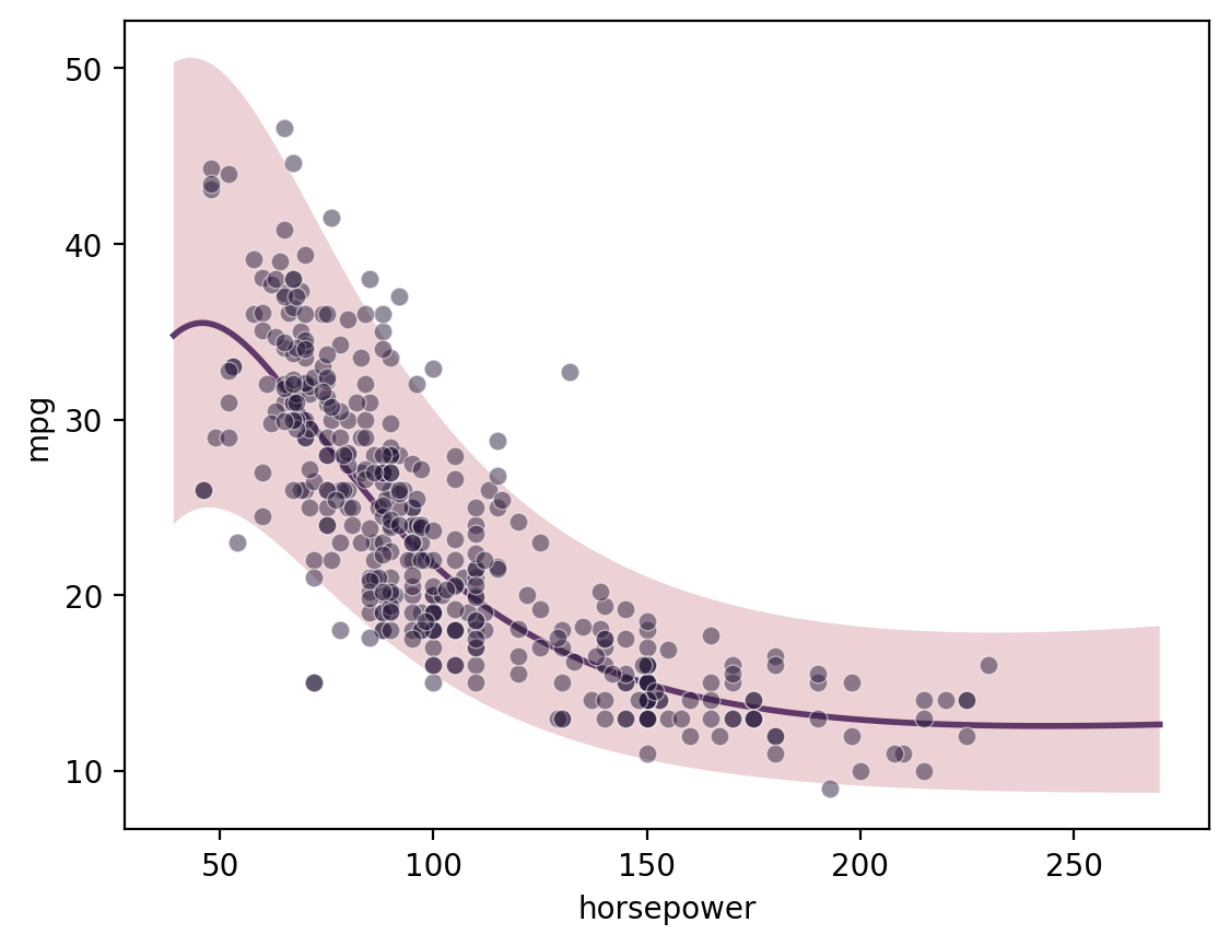
Single-output regression

gp = GP(ds)
gp.fit(outputs=['mpg'], continuous_dims=['horsepower'], continuous_kernel='RBF', seed=0, ARD=True)

X = gp.prepare_grid()
y = gp.predict_grid();

pp = gmb.ParrayPlotter(X, y)
pp.plot()
sns.scatterplot(data=cars, x='horsepower', y='mpg', color=sns.cubehelix_palette()[-1], alpha=0.5);

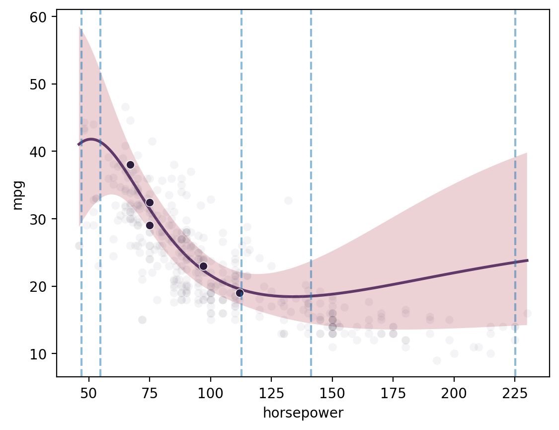
Batch single-task proposals with qNEI

Botorch uses “q Noisy Expected Improvement” (qNEI) to select a batch of points to evaluate. This is now controlled through a simple method propose, which maximizes the output by default. Set maximize=False to minimize instead.

ds2 = gmb.DataSet(
    cars.sample(5, random_state=1),
    outputs=["mpg", "acceleration"],
    log_vars=["mpg", "acceleration", "weight", "horsepower", "displacement"],
)

gp = GP(ds2)
gp.fit(
    outputs=["mpg"],
    continuous_dims=["horsepower"],
    continuous_kernel="RBF",
    seed=0,
    ARD=True,
)

X = gp.prepare_grid(
    limits=gmb.parray(
        horsepower=[ds.wide.horsepower.min(), ds.wide.horsepower.max()], stdzr=gp.stdzr
    )
)
y = gp.predict_grid()

sns.scatterplot(data=cars, x='horsepower', y='mpg', color=sns.cubehelix_palette()[-1], alpha=0.05);
pp = gmb.ParrayPlotter(X, y)
pp.plot()
sns.scatterplot(
    data=ds2.wide, x="horsepower", y="mpg", color=sns.cubehelix_palette()[-1]
)

bounds = np.array([[X.z.values().min(0)+0.1, X.z.values().max(0)-0.1]]).T
# bounds = torch.from_numpy(bounds).to(gp.device)

candidates, _ = gp.propose(maximize=True, q=5, bounds=bounds)

for x in candidates:
    plt.axvline(x.values(), color='C0', linestyle='--', alpha=0.5)

/home/john/mambaforge/envs/gumbi-test/lib/python3.11/site-packages/botorch/optim/optimize.py:652: RuntimeWarning: Optimization failed in `gen_candidates_scipy` with the following warning(s):
[OptimizationWarning('Optimization failed within `scipy.optimize.minimize` with status 2 and message ABNORMAL: .')]
Trying again with a new set of initial conditions.
  return _optimize_acqf_batch(opt_inputs=opt_inputs)
/home/john/mambaforge/envs/gumbi-test/lib/python3.11/site-packages/botorch/optim/optimize.py:652: RuntimeWarning: Optimization failed on the second try, after generating a new set of initial conditions.
  return _optimize_acqf_batch(opt_inputs=opt_inputs)

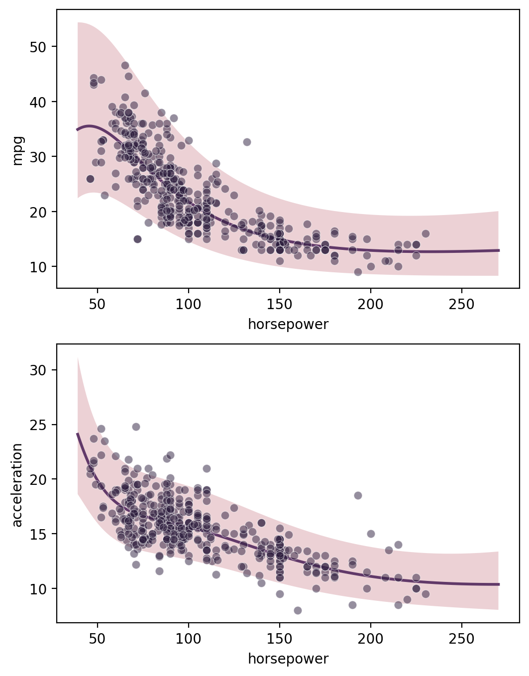
Multi-output regression

gp = GP(ds)
gp.fit(outputs=['mpg', 'acceleration'], continuous_dims=['horsepower'], multitask_kernel='Hadamard')

X = gp.prepare_grid()
Y = gp.predict_grid()

axs = plt.subplots(2,1, figsize=(6, 8))[1]
for ax, output in zip(axs, gp.outputs):
    y = Y.get(output)

    gmb.ParrayPlotter(X, y).plot(ax=ax)

    sns.scatterplot(data=cars, x='horsepower', y=output, color=sns.cubehelix_palette()[-1], alpha=0.5, ax=ax);

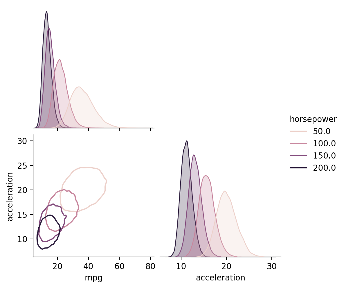
Learned correlations between outputs

X = gp.parray(horsepower=[50, 100, 150, 200])
gp.predict_points(X)
y = gp.predictions

samples_df = pd.concat(
    [
        pd.DataFrame(point.dist.rvs(10000, random_state=j).as_dict()).assign(
            horsepower=hp.values()
        )
        for j, (point, hp) in enumerate(zip(y, X))
    ],
    ignore_index=True,
)

sns.pairplot(
    samples_df, hue="horsepower", kind="kde", corner=True, plot_kws={"levels": 1}
)

<seaborn.axisgrid.PairGrid at 0x7f15ec665690>

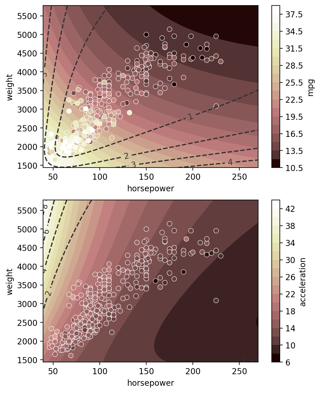
Multi-input multi-output regression

gp = GP(ds)

# multitask_kernels = ['Independent', 'Hadamard', 'Kronecker']
gp.fit(outputs=['mpg', 'acceleration'], continuous_dims=['horsepower', 'weight'], multitask_kernel='Hadamard');

XY = gp.prepare_grid()
Z = gp.predict_grid(with_noise=False)

X = XY["horsepower"]
Y = XY["weight"]

axs = plt.subplots(2,1, figsize=(6, 8))[1]
for ax, output in zip(axs, gp.outputs):
    z = Z.get(output)
    μ = z.μ
    σ = z.dist.std()
    norm = plt.Normalize(μ.min(), μ.max())

    plt.sca(ax)
    pp = gmb.ParrayPlotter(X, Y, z)
    pp(plt.contourf, levels=20, cmap="pink", norm=norm)
    pp.colorbar(ax=ax)

    cs = ax.contour(
        X.values(), Y.values(), σ, levels=4, colors="0.2", linestyles="--"
    )
    ax.clabel(cs)

    sns.scatterplot(
        data=cars,
        x="horsepower",
        y="weight",
        hue=output,
        palette="pink",
        hue_norm=norm,
        ax=ax,
    )
    ax.legend().remove()

    # title = "Automatic Relevance Detection" if ard else "Joint Kernel"
    # ax.set_title(title)

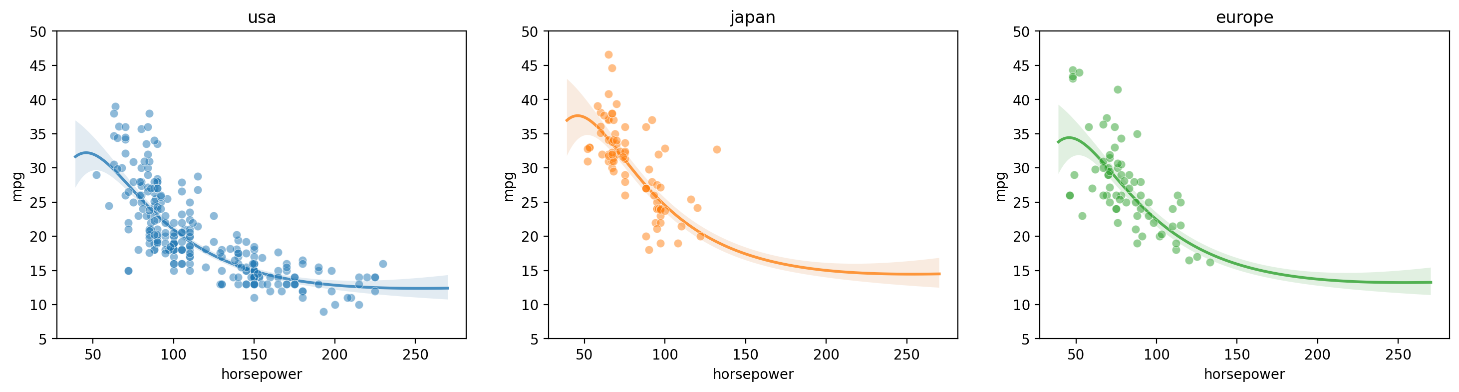
Mixed categorical-continuous regression

gp = GP(ds)
gp.fit(outputs=['mpg'], categorical_dims=['origin'], continuous_dims=['horsepower']);

X = gp.prepare_grid()
axs = plt.subplots(1,3, figsize=(18, 4))[1]
for i, (ax, origin) in enumerate(zip(axs, cars.origin.unique())):
    y = gp.predict_grid(categorical_levels={'origin': origin}, with_noise=False)

    gmb.ParrayPlotter(X, y).plot(ax=ax, palette=sns.light_palette(f'C{i}'))

    sns.scatterplot(data=cars[cars.origin==origin], x='horsepower', y='mpg', color=f'C{i}', alpha=0.5, ax=ax);
    ax.set_title(origin)
    ax.set_ylim([5, 50])

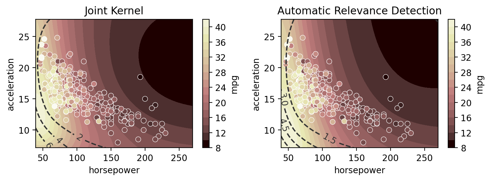
Multi-input regression

Here we compare the use of “Automatic Relevance Determination” (ARD) - using independent length scales for each input dimension - to a single length scale for all input dimensions. ARD is on by default in gumbi but off by default in AssayOptimizer (in which it’s controlled by the isotropic argument - True by default). We can see below that ARD learns that the output changes more rapidly in response to a small change in horsepower relative to mpg, as reflected by the more eliptical contours in comparison to the more circular contours of the non-ARD model.

from matplotlib.colors import Normalize as cNormalize
norm = cNormalize()
norm(ds.wide.mpg);

ds3 = gmb.DataSet(
    cars,
    outputs=["mpg"],
    log_vars=["mpg", "acceleration", "weight", "horsepower", "displacement"],
)

gp = GP(ds3)

axs = plt.subplots(1, 2, figsize=(8, 3))[1]
for ax, ard in zip(axs, [False, True]):

    gp.fit(outputs=["mpg"], continuous_dims=["horsepower", "acceleration"], ARD=ard)

    XY = gp.prepare_grid()
    X = XY["horsepower"]
    Y = XY["acceleration"]
    z = gp.predict_grid(with_noise=False)
    μ = z.μ
    σ = z.dist.std()

    plt.sca(ax)
    pp = gmb.ParrayPlotter(X, Y, z)
    pp(plt.contourf, levels=20, cmap="pink", norm=norm)
    pp.colorbar(ax=ax)

    cs = ax.contour(
        X.values(), Y.values(), σ, levels=4, colors="0.2", linestyles="--"
    )
    ax.clabel(cs)

    sns.scatterplot(
        data=cars,
        x="horsepower",
        y="acceleration",
        hue="mpg",
        palette="pink",
        hue_norm=norm,
        ax=ax,
    )
    ax.legend().remove()

    title = "Automatic Relevance Detection" if ard else "Joint Kernel"
    ax.set_title(title)

plt.tight_layout()

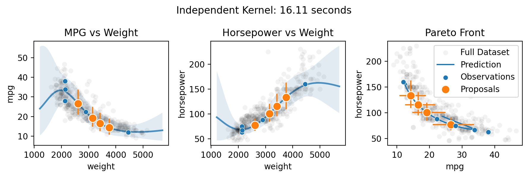
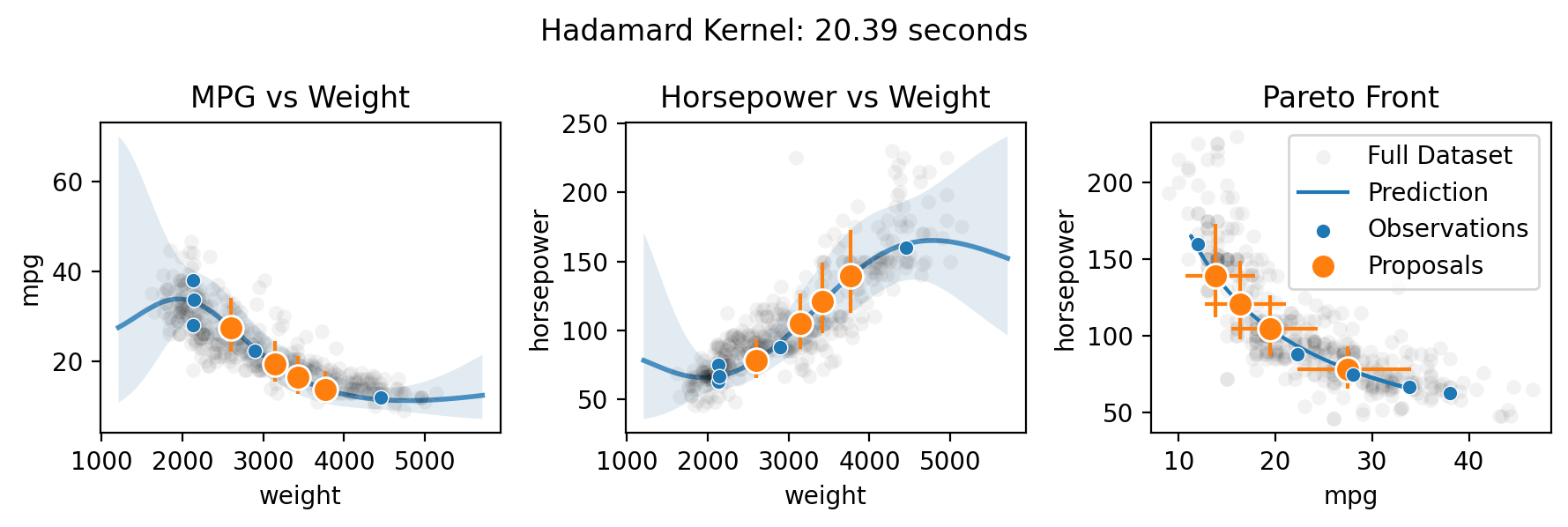
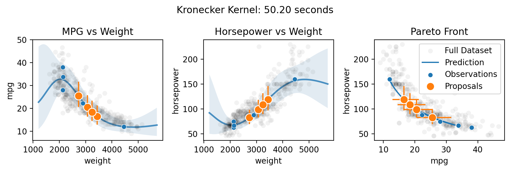
Multi-output (Pareto front) optimization with qNEHVI

Finally, Botorch can natively optimize the Pareto front of the multiple objectives. Here we take the toy scenario of wanting to select the ideal weight for a car in order to maximize both its fuel efficiency and horsepower.

There are three methods for specifying the multitask kernel: Independent, Hadamard, and Kronecker. Hadamard and Kronecker learn a correlation between the outputs, while Independent simply builds separate GPs for each output. The Kronecker kernel requires all outputs to be observed at every input, while the Hadamard kernel does not. Practically, the Hadamard kernel may perform better in low output and input dimensions (it’s the default for two or fewer outputs), while the Kronecker kernel supposedly may perform better in higher output dimensions (it’s the default for three or more outputs) and the Independent kernel may perform better in high input dimensions with relatively few observations. The choice can be forced by setting the multitask_kernel argument to either "Independent", "Kronecker", or "Hadamard".

import time

q = 4

ds4 = gmb.DataSet(
    cars.sample(5, random_state=0),
    outputs=["mpg", "horsepower", "acceleration", "displacement", "model_year"],
    log_vars=["mpg", "acceleration", "weight", "horsepower", "displacement"],
)

gp = GP(ds4)

for multitask_kernel in ["Independent", "Hadamard", "Kronecker"]:

    start = time.time()
    gp.fit(
        outputs=["mpg", "horsepower"],
        continuous_dims=["weight"],
        continuous_kernel="RBF",
        seed=0,
        ARD=True,
        multitask_kernel=multitask_kernel,
    )

    candidates, _ = gp.propose(q=q)
    preds = gp.predict_points(candidates)

    X = gp.prepare_grid()
    Y = gp.predict_grid()
    end = time.time()

    axs = plt.subplots(1, 3, figsize=(9, 3))[1]
    for ax, output in zip(axs, gp.outputs):
        y = Y.get(output)

        sns.scatterplot(data=cars, x="weight", y=output, color="k", alpha=0.05, ax=ax)

        gmb.ParrayPlotter(X, y).plot(ax=ax, palette=sns.light_palette("C0"))

        for weight, pred in zip(candidates, preds):
            y = pred.get(output).μ
            y_err = np.abs(np.array([pred.get(output).dist.interval(0.95)]) - y).T
            ax.errorbar(weight, y, y_err, fmt="o", color="C1", ms=10, mec="w")

        sns.scatterplot(
            data=ds4.wide, x="weight", y=output, color="C0", ax=ax, zorder=10
        )

    ax = axs[2]
    sns.scatterplot(
        data=cars,
        x="mpg",
        y="horsepower",
        ax=ax,
        color="k",
        alpha=0.05,
        label="Full Dataset",
    )
    ax.plot(Y.get("mpg").μ, Y.get("horsepower").μ, label="Prediction", color="C0")

    x = preds.get("mpg").μ
    y = preds.get("horsepower").μ
    x_err = np.abs(np.array(preds.get("mpg").dist.interval(0.95)) - x)
    y_err = np.abs(np.array(preds.get("horsepower").dist.interval(0.95)) - y)
    ax.errorbar(
        x, y, y_err, x_err, fmt="o", color="C1", ms=10, label="Proposals", mec="w"
    )

    sns.scatterplot(
        data=ds4.wide,
        x="mpg",
        y="horsepower",
        ax=ax,
        label="Observations",
        color="C0",
        zorder=10,
    )
    ax.legend()

    axs[0].set_title("MPG vs Weight")
    axs[1].set_title("Horsepower vs Weight")
    axs[2].set_title("Pareto Front")
    plt.suptitle(f"{multitask_kernel} Kernel: {end-start:.2f} seconds")
    plt.tight_layout()

/home/john/mambaforge/envs/gumbi-test/lib/python3.11/site-packages/botorch/optim/optimize.py:652: RuntimeWarning: Optimization failed in `gen_candidates_scipy` with the following warning(s):
[OptimizationWarning('Optimization failed within `scipy.optimize.minimize` with status 2 and message ABNORMAL: .')]
Trying again with a new set of initial conditions.
  return _optimize_acqf_batch(opt_inputs=opt_inputs)
/home/john/mambaforge/envs/gumbi-test/lib/python3.11/site-packages/botorch/optim/optimize.py:652: RuntimeWarning: Optimization failed on the second try, after generating a new set of initial conditions.
  return _optimize_acqf_batch(opt_inputs=opt_inputs)
/home/john/mambaforge/envs/gumbi-test/lib/python3.11/site-packages/botorch/optim/optimize.py:652: RuntimeWarning: Optimization failed in `gen_candidates_scipy` with the following warning(s):
[OptimizationWarning('Optimization failed within `scipy.optimize.minimize` with status 2 and message ABNORMAL: .')]
Trying again with a new set of initial conditions.
  return _optimize_acqf_batch(opt_inputs=opt_inputs)